Category Archives: Techniques

In-focus Region Detection Using Harmonic Variance of DCT Band-pass Filtering

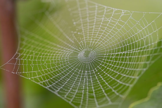
Detecting in-focus regions in a low depth-of-field (DoF) image has important applications in scene understanding, object-based coding, image quality assessment and depth estimation because such regions may indicate semantically meaningful objects.

Here I show a challenging example,  a spider web. Note that some parts of the defocus regions still demonstrate strong patch variances.

spider-web-macro-photography

In our paper, we show that by simply using DCT band-pass filtering and harmonic variance, we could get very robust in-focus measurement, as shown in the following picture. The idea is simple. Defocus regions only cover some low frequency bands because of lens blur, while in-focus region cover the full spectrum bands. By using DCT band-pass filtering, we could extract those frequency responses. If we just sum those responses all together, the final estimate could be well biased due to very high responses of just some low frequency channels. Harmonic mean solves this problem by penalizing those outliers and could generate very robust outputs.

hv

In short, this algorithm works by
1) apply 63 DCT band-pass filtering (for 8×8 patches) to the input image, excluding the first DC/average filtering
2) compute patch variance for each 63 filtered images. Now at every pixel location (x, y), we have 63 variance measurements
3) compute harmonic mean of these 63 variance as harmonic variance
4) optionally, we could apply sigmoid function to the harmonic variance image to restrict the outputs to be [0, 1].

If you want to estimate the actual noise level of the input image, please refer to our paper for kurtosis analysis.

import numpy as np
import scipy.misc as misc
import scipy.ndimage as ndimage
import scipy.stats as stats
import matplotlib.pyplot as plt

def Sigmoid(x, ratio) :
    return 1 / (1 + np.exp(-ratio * x) )

def Tanh(x, ratio) :
    return 2 * Sigmoid(2 * x, ratio) - 1

def GenerateDCT8x8Base() :

    N = 8
    x = np.array( np.arange(0, N ), dtype=np.float32, ndmin=2 )

    C = np.cos( np.transpose(2*x+1) * x * np.pi / (2.0*N) ) * np.sqrt(2.0/N)
    C[:, 0] = C[:, 0] / np.sqrt(2.0)

    plt.close('all')
    plt.figure()

    filters = []
    for i in range( N ) :
        for j in range( N ) :

            X = np.transpose(np.array(C[:, i], ndmin=2)) * np.transpose( C[:, j])
            im = misc.imresize(X, (128, 128), interp='nearest')
            plt.subplot(N, N, i * N + j + 1)
            plt.imshow(im, cmap=plt.cm.gray)
            plt.axis('off')

            filters.append( X )

    del filters[0] 

    return filters

def ComputeHarmonicVariance(im, kernels):

    size = list(im.shape)
    size.append(len(kernels))

    k_size = kernels[0].shape
    k_avg = np.ones( k_size, np.float32) / (k_size[0] * k_size[1])

    outs = np.empty( size, dtype=np.float32)
    for i in range(len(kernels)) :
        data = ndimage.convolve(im, kernels[i])
        data2 = data * data

        EX2 = ndimage.convolve(data2, k_avg)
        E2X = np.square(ndimage.convolve(data, k_avg))

        outs[:,:,i] = EX2 - E2X

    variance = np.empty( im.shape, dtype=np.float32 )
    for y in range(size[0]):
        for x in range(size[1]):
            data = outs[y, x, :]
            variance[y, x] = stats.hmean(outs[y,x,:]+1e-8)

    return variance            

im = misc.imread('Spider-Web-Macro-Photography.jpg').astype(np.float32)
im = im[:,:,0] # extract Red channel for demonstration
kernels = GenerateDCT8x8Base()
hv = ComputeHarmonicVariance(im, kernels)
plt.figure(), plt.imshow(Tanh(hv, 0.01), cmap=plt.cm.gray), plt.title('hv t 0.01')
Advertisement

A simple implementation of sobel filtering in Python

One can directly use ‘ndimage’ of scipy to compute the sobel filtering of the input image as follows:

dx = ndimage.sobel(im, 0)  # horizontal derivative
dy = ndimage.sobel(im, 1)  # vertical derivative
mag = np.hypot(dx, dy)  # magnitude
mag *= 255.0 / np.max(mag)  # normalize

Or your can write the function by yourself and add more features to it.

def sobel_filter(im, k_size):
    
    im = im.astype(np.float)
    width, height, c = im.shape
    if c > 1:
        img = 0.2126 * im[:,:,0] + 0.7152 * im[:,:,1] + 0.0722 * im[:,:,2]
    else:
        img = im
    
    assert(k_size == 3 or k_size == 5);
    
    if k_size == 3:
        kh = np.array([[-1, 0, 1], [-2, 0, 2], [-1, 0, 1]], dtype = np.float)
        kv = np.array([[1, 2, 1], [0, 0, 0], [-1, -2, -1]], dtype = np.float)
    else:
        kh = np.array([[-1, -2, 0, 2, 1], 
                   [-4, -8, 0, 8, 4], 
                   [-6, -12, 0, 12, 6],
                   [-4, -8, 0, 8, 4],
                   [-1, -2, 0, 2, 1]], dtype = np.float)
        kv = np.array([[1, 4, 6, 4, 1], 
                   [2, 8, 12, 8, 2],
                   [0, 0, 0, 0, 0], 
                   [-2, -8, -12, -8, -2],
                   [-1, -4, -6, -4, -1]], dtype = np.float)
    
    gx = signal.convolve2d(img, kh, mode='same', boundary = 'symm', fillvalue=0)
    gy = signal.convolve2d(img, kv, mode='same', boundary = 'symm', fillvalue=0)

    g = np.sqrt(gx * gx + gy * gy)
    g *= 255.0 / np.max(g)
  
    #plt.figure()
    #plt.imshow(g, cmap=plt.cm.gray)      
  
    return g

Save Image into PPM ASCII Format in Matlab and Python

Here I wrote a function to save image/matrix into PPM format. I tried to simplify the saving process by using the matlab function ‘dlmwrite’ such that I only need to write the header for this PPM format. However, before streaming the image data, different channels of the input image must be interleaved. I experimented two ways to do this. Both work just fine, and the use of matlab function ‘cat’ (or ‘permute’) make the implementation very simple.

function write_ppm(im, fname, xval)

[height, width, c] = size(im);
assert(c == 3);

fid = fopen( fname, 'w' );

%% write headers
fprintf( fid, 'P3\n' );
fprintf( fid, '%d %d\n', width, height);
fprintf( fid, '%d \n', xval); %maximum values

fclose( fid ); 

%% interleave image channels before streaming
c1 = im(:, :, 1)';
c2 = im(:, :, 2)';
c3 = im(:, :, 3)';
im1 = cat(2, c1(:), c2(:), c3(:));

%% data streaming, could be slow if the image is large
dlmwrite(fname, int32(im1), '-append', 'delimiter', '\n')

The implementation in Python is even simpler. ‘f.write()’ is capable of writing the entire image in one function call with the help of ‘\n’.join().

def write_ppm(fname, im, xval):
    
    height, width, nc = im.shape
    assert nc == 3
    
    f = open(fname, 'w')
    
    f.write('P3\n')
    f.write(str(width)+' '+str(height)+'\n')
    f.write(str(xval)+'\n')
    
    # interleave image channels before streaming    
    c1 = np.reshape(im[:, :, 0], (width*height, 1))
    c2 = np.reshape(im[:, :, 1], (width*height, 1))
    c3 = np.reshape(im[:, :, 2], (width*height, 1))
    
    im1 = np.hstack([c1, c2, c3])
    im2 = im1.reshape(width*height*3)

    f.write('\n'.join(im2.astype('str')))
    f.write('\n')

    f.close()

Phase difference calculation for Phase Detection Autofocus (PDAF)

Phase Detection Autofocus (PDAF) is one of the key advantages of D-SLR cameras over conventional Point-and-Shoot cameras, which usually employ contrast based autofocus system by sweeping through the focal range and stopping at the point where maximum contrast is detected. A good tutorial about how PDAF works can be found @ http://photographylife.com/how-phase-detection-autofocus-works.

In the following, I show how to find the phase difference in Python when two separate distributions are obtained from two separate AF sensors corresponding to one particular AF point. The function ‘correlate’ actually does a brute-force search in the entire phase shift space and returns a phase shift value which corresponds to the maximum correlation value.

import numpy as np
from scipy import signal

def gaussian(x, mu, sig):
    return np.exp(-np.power(x - mu, 2.) / 2 * np.power(sig, 2.))

n_ele = 100
dt = np.linspace(0, 10, n_ele)
g1 = gaussian(dt, 2, 1.3)
g2 = gaussian(dt, 6, 2.2)

#Cross-correlation of two 1-dimensional sequences. This function 
# computes the correlation as generally defined in signal 
# processing texts: z[k] = sum_n a[n] * conj(v[n+k])
# with a and v sequences being zero-padded where necessary 
# and conj being the conjugate
xcorr = signal.correlate(g1, g2)

# The peak of the cross-correlation gives the shift between the 
# two signals The xcorr array goes from -nsamples to nsamples
dt2 = np.linspace(-dt[-1], dt[-1], 2 * n_ele - 1)
print 'phase shift: ', dt2[xcorr.argmax()]

Interested readers are encouraged to read more about phase difference calculation @ http://stackoverflow.com/questions/6157791/find-phase-difference-between-two-inharmonic-waves

To accelerate the calculation, people usually transform this problem into Fourier domain to determine the phase correlation between two PDAF sensors, which is also a general technique for translation, rotation, and scale-invariant image registration. For example, given the following two images, with only translational movement between them,

trans_t2trans_t1

one can compute the phase correlation between the two input images as:

import numpy as np
from scipy import misc
import matplotlib.pyplot as plt

def rgb2gray(rgb):
    return np.dot(rgb[...,:3], [0.299, 0.587, 0.144])

im1 = misc.imread('trans_t2.png')
im2 = misc.imread('trans_t1.png')

img1 = rgb2gray(im1).astype(np.float)
img2 = rgb2gray(im2).astype(np.float)

f1 = np.fft.fftshift(np.fft.fft2(img1))
f2 = np.fft.fftshift(np.fft.fft2(img2))

tmp1 = np.multiply(f1, np.conjugate(f2))
tmp2 = np.abs(np.multiply(f1, f2))
tmp3 = np.abs(np.fft.ifft2(tmp1 / tmp2))

translation = np.unravel_index(np.argmax(tmp3), tmp3.shape)
print translation

For more details, please refer to :
Reddy, B. S. and Chatterji, B. N., An FFT-Based Technique for Translation, Rotation, and Scale-Invariant Image Registration, IEEE Transactions on Image Processing, Vol. 5, No. 8, August 1996.

Matplotlib savefig without border/frame

For some cases, the function ‘savefig’ with ‘bbox_inches=’tight” doesn’t work well and still generates images with borders that you want to remove.

plt.savefig('fn.jpg', dpi = 300, bbox_inches='tight')

One way to avoid this is to look into the axes properties before calling the function ‘savefig’. Basically, you just need to create an axes object without border/frame and add it to the pre-generated figure window.

def save_image(data, cm, fn):
  
    sizes = np.shape(data)
    height = float(sizes[0])
    width = float(sizes[1])
    
    fig = plt.figure()
    fig.set_size_inches(width/height, 1, forward=False)
    ax = plt.Axes(fig, [0., 0., 1., 1.])
    ax.set_axis_off()
    fig.add_axes(ax)

    ax.imshow(data, cmap=cm)
    plt.savefig(fn, dpi = height) 
    plt.close()

Kile can not edit tex file

Sometimes when I use Kile to open tex files, kile just simply cannot edit them. I can move the cursor freely but cannot type in anything. In this case, you just need to uncheck Tools -> Read Only Mode.

If the read-only problem is caused by ‘The file xxx.tex was opened and contained too long lines (more than 1 024 characters). Too long lines were wrapped and the document is set to read-only mode, as saving will modify its content.’, you may walk around this by setting the line lenght to 0, under Settings -> Configure Kile -> Open/Save -> Line Lenght Limit.

The wield case I met is that my kile didn’t have menu bar, although kate has that. I searched online and found out that you can re-enable the menu bar by editing the kilerc under ~/.kde/share/config/. Changing ‘menubar=Disabled’ to ‘Enabled’ would make the menu bar re-appear.

write DICOM images from a 3D array

To write a DICOM image sequence from a 3D data array using MATLAB, you will need to specify ‘PixelSpacing’ and the ‘SliceThickness’, otherwise the 3D reconstruction software would have no idea to determine the length of the volume data. One way is to copy a sample metadata structure from another volume, update it with the new  ‘PixelSpacing’ and ‘SliceThickness’,  and pass it to dicomwrite. dicomwrite can write the correct ‘PixelSpacing’ and ‘SliceThickness’ into the dicom file, however, the reconstruction software (for example, slicer) would still treat ‘SliceThickness’ as 1 even it displays the correct ‘SliceThickness’ value. Another way is to directly specify these matadata values as the following. You just need to find the corresponding SOP Class UID for your dicom data from http://www.apteryx.fr/dicom/dicom_conformance


% T defines the 'PixelSpacing' and the 'SliceThickness'

%% save dicom images
for i = 1 : n_slices

    status = dicomwrite(uint16(data(:,:,i)), ...
    file_name, ...
    'SliceThickness', T(3), ...
    'PixelSpacing', [T(1); T(2)], ...
    'SliceLocation', location_base - (i-1)*T(3), ...
    'ImageOrientationPatient', [1 0 0 0 1 0], ...
    'CreateMode', 'Copy', ...
    'SOPClassUID', '1.2.840.10008.5.1.4.1.1.2');

end

Show the input data for the accumulating function of Matlab accumarray

When using MATLAB accumarray, if the subscripts in 'subs' are not sorted, the accumulating function ‘fun‘ should not depend on the order of the values in its input data. Otherwise you would have weird results. To show the input data for the accumulating function, one can define the function as ‘@(x){x}’. This would save the input data for you. For example,

>> val = 101:105;
>> subs = [1; 2; 4; 2; 4]
>> A = accumarray(subs, val, [], @(x){x})

A =

[       101]
[2x1 double]
[]
[2x1 double]

Converting STL surface mesh to volume mesh using GMSH

Just three simple steps:
> File -> Merge -> “filename.stl”
> Geometry -> Elementary entities -> Add -> New -> Volume, click on the surface to build the volume
> Mesh -> 3D

Sample STL file can be downloaded @ https://geuz.org/trac/gmsh/attachment/wiki/STLRemeshing/pelvis.stl.gz (user name and password are ‘gmsh’ ‘gmsh’.)

If some errors happened, it is the problem of your input stl surface mesh. One common error is “self intersecting surface mesh, computing intersections (this could tak a while)”. If your surface is generated by some segmentation software and too complicated to fix. You may want to convert your surface mesh to a solid volume and then rebuild the surface mesh through isosurface reconstruction.

Or you can use meshlab to find those problematic faces and edges. Use the tools from Filters/Selection/Select Self Intersecting Faces (Select non Manifold Edges) to select these regions, delete them, and then use hole filling tool to generate the final surface mesh. This sometimes can solve some weird volume mesh problems, for example, volume mesh outside the surface mesh.

http://www.geuz.org/pipermail/gmsh/2010/005558.html

—————————–

[10/27/2014] Instead of using GMSH, I actually used TetGen (http://wias-berlin.de/software/tetgen/) for several of my projects for volume mesh generation. It is a great tool for its simple syntax and lots of easy to understand examples. It was also integrated into Febio (http://mrl.sci.utah.edu/software/febio/), a FEM analysis software for biomechanical simulations. A paper of using both TetGen and Febio can be found here.